Books › AI Foundations: from zero

Inside a neural network: structure, learning and updates

By Kapil Kumar Gupta

The idea in one breath

In Chapter 4 you met the neuron: a tiny voter that multiplies clues by weights, adds a nudge, and decides. A network is many of them. Learning means finding good numbers for all the weights.

This deep dive follows one single learning step on a very small network, with every number written out. If you can follow this, you can follow how a network with a billion weights learns, because the only difference is how many numbers there are.

The structure

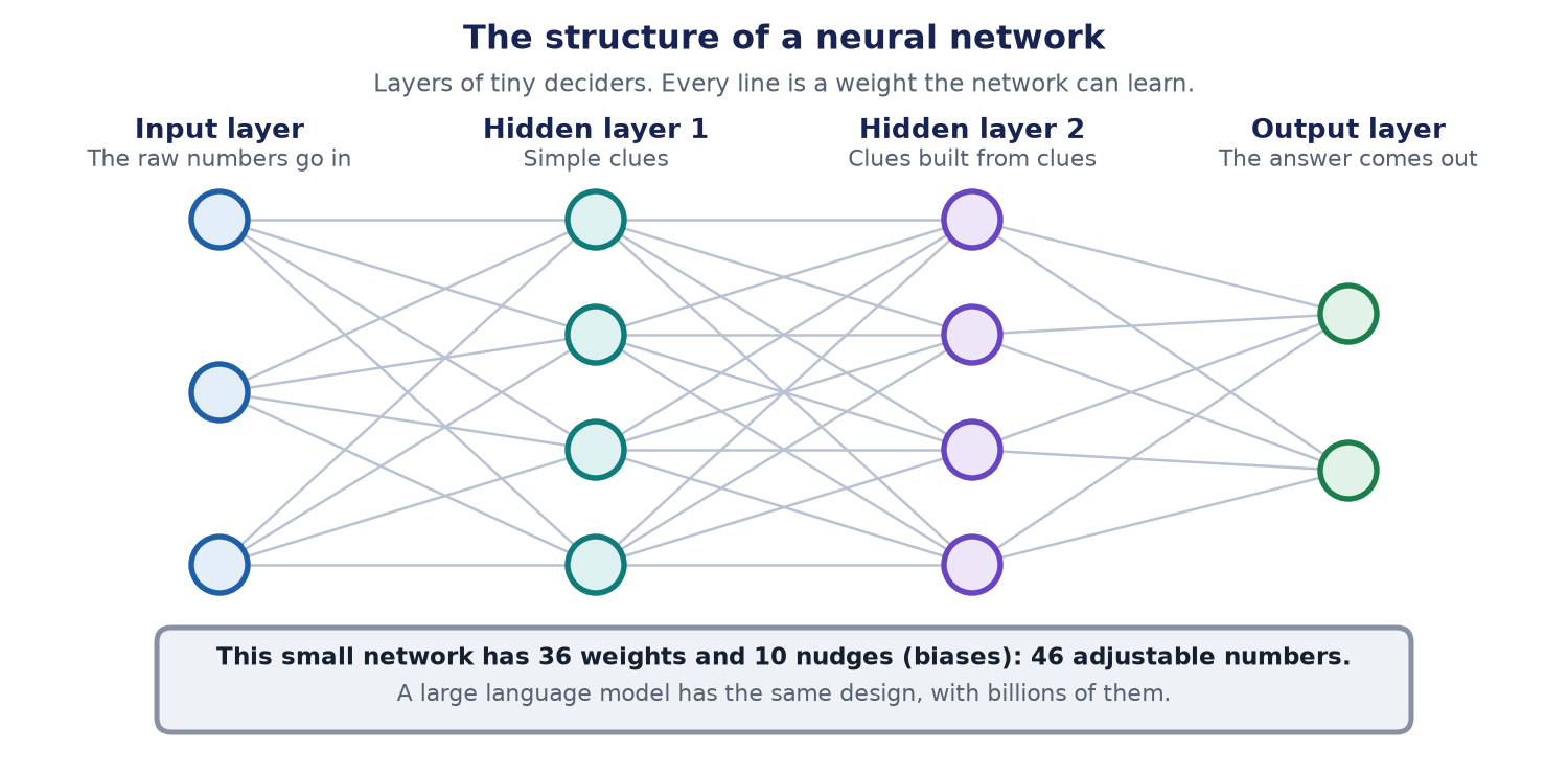
A network is arranged in layers. Every circle in one layer is joined to every circle in the next. Each line carries a weight. Each circle also has a nudge, called its bias.

• The input layer holds the raw numbers, such as the dots of a photo or the numbers that stand for a word.
• The hidden layers are in the middle. "Hidden" only means we do not directly see their values.
• The output layer gives the answer.

How many numbers can a network learn? Count the lines and the nudges. The network in the picture has 3 × 4 + 4 × 4 + 4 × 2 = 36 weights and 4 + 4 + 2 = 10 nudges: 46 numbers. These numbers are called parameters. A language model has the same design with billions of them.

Two words you will meet: the width of a layer is how many circles it has, and the depth of a network is how many layers it has. More of either gives the network more room to learn, and costs more to run.

A network small enough to hold in your head

Now the worked example. We use a tiny network with two inputs, two hidden circles and one output. The numbers are chosen to make the arithmetic easy.

• The inputs are 1 and 2.
• Hidden circle 1 has weights 0.5 and 0.25, and a nudge of 0.
• Hidden circle 2 has weights −1.0 and 0.5, and a nudge of 0.5.
• The output has weights 0.6 and 0.4, and a nudge of 0.
• The right answer, the target, is 1.0.

The decide step in the hidden circles is ReLU: if the total is below zero, output zero; otherwise output the total itself.

Step 1: the forward pass

Numbers flow from left to right.

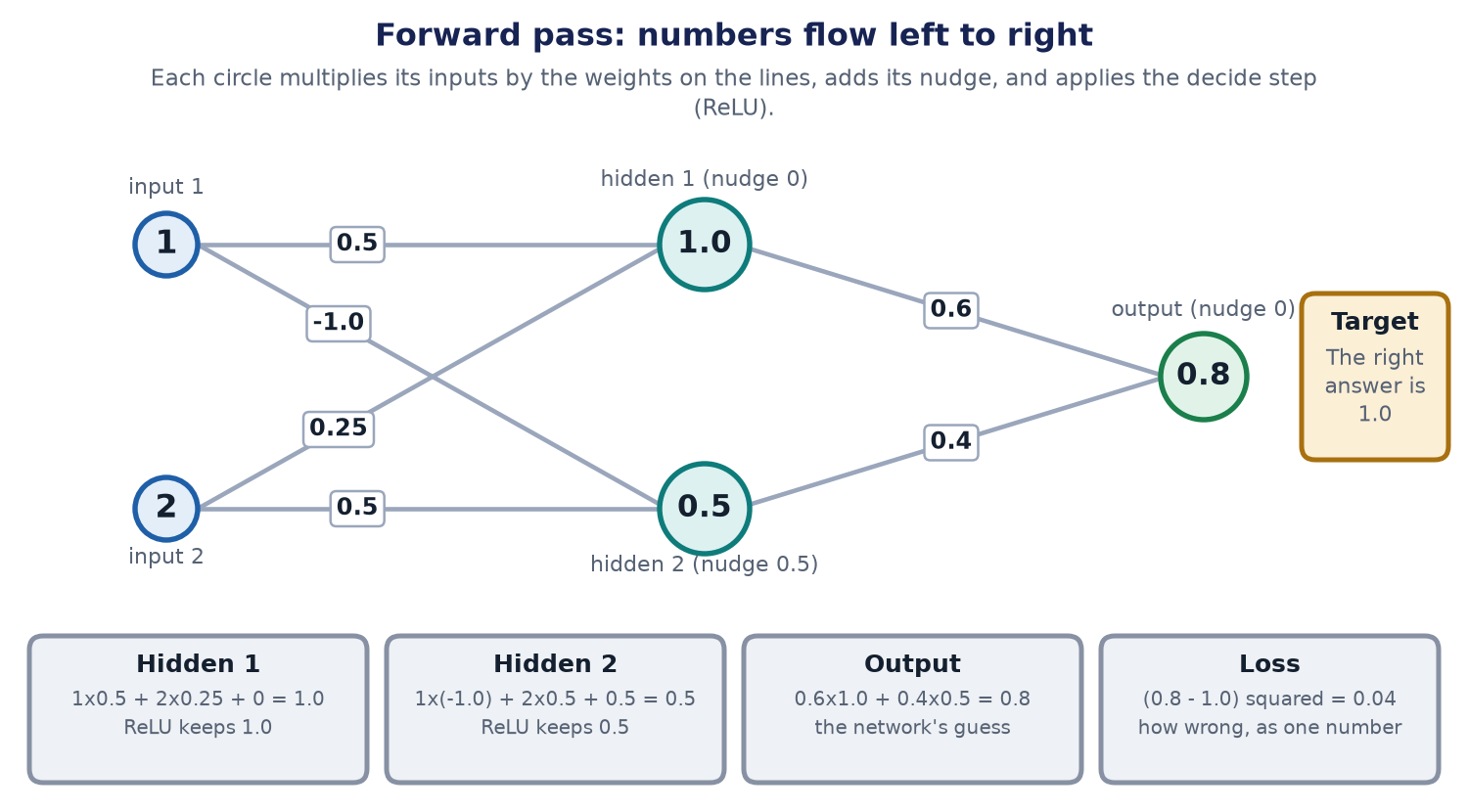
• Hidden 1: 1 × 0.5 + 2 × 0.25 + 0 = 1.0. ReLU keeps it: 1.0.
• Hidden 2: 1 × (−1.0) + 2 × 0.5 + 0.5 = 0.5. ReLU keeps it: 0.5.
• Output: 0.6 × 1.0 + 0.4 × 0.5 + 0 = 0.8.

The network guessed 0.8. The right answer is 1.0. It is too low.

Step 2: the loss

We need one number that says how wrong the guess is. That number is the loss. A common choice is the squared difference:

loss = (guess − target)² = (0.8 − 1.0)² = 0.04

Squaring does two useful things. It makes the loss positive whether the guess is too high or too low, and it punishes big mistakes much more than small ones: being off by 2 costs 4, being off by 0.2 costs only 0.04.

Different jobs use different loss recipes. For choosing between classes (such as order, question or complaint), a popular one is cross-entropy. In plain words, it punishes the network hardest when it is confidently wrong. A network that says "99% sure it is a question" when it is a complaint is scored much worse than one that says "55% sure". That nudges the network to be honest about its doubts.

The aim of all learning is to make the loss small.

Step 3: backpropagation, passing the blame back

Now the key question: for each weight, if I make it a little bigger, does the loss go up or down, and by how much? That number is the weight's gradient. Think of it as a slope. A negative gradient says "make this weight bigger and the loss falls".

You could find each gradient by trying a tiny change to every weight, one at a time. With a billion weights that would take forever. Backpropagation is the clever shortcut: start at the error and pass the blame backwards, layer by layer, reusing work as you go.

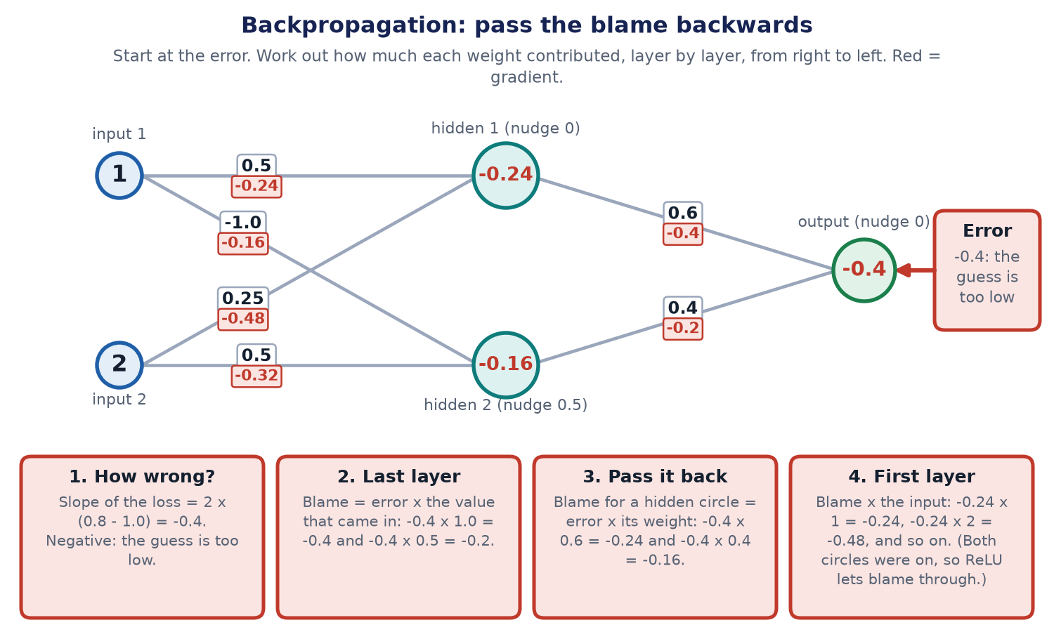
1. How wrong? The slope of the loss is 2 × (0.8 − 1.0) = −0.4. (This is the rule for the squared loss: twice the difference.) Negative means: the guess is too low, so we want the output to go up. 2. The last layer's weights. The gradient of a weight is the blame times the value that came in along that line. For the weight 0.6, the value that came in was 1.0, so its gradient is −0.4 × 1.0 = −0.4. For the weight 0.4, the value was 0.5, so −0.4 × 0.5 = −0.2. The output's own nudge gets the blame itself: −0.4. 3. Pass the blame back. How much blame goes to each hidden circle? The error times the weight that connects it: −0.4 × 0.6 = −0.24 for circle 1, and −0.4 × 0.4 = −0.16 for circle 2. 4. The first layer's weights. ReLU lets blame through when its circle was switched on, and both were. So the gradient for each weight is the circle's blame times the input on that line: for circle 1, −0.24 × 1 = −0.24 and −0.24 × 2 = −0.48; for circle 2, −0.16 × 1 = −0.16 and −0.16 × 2 = −0.32. The nudges get −0.24 and −0.16.

The pattern is the same at every layer: *blame in, times what came in, gives the gradient; blame times the weight gives the blame to pass back.* This is the whole trick, and it works for networks of any size.

Step 4: the update

Now change every weight a little, in the direction that lowers the loss:

new weight = old weight − learning rate × gradient

The learning rate says how big a step to take. Here it is 0.1.

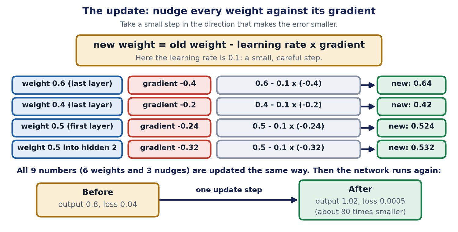
• Weight 0.6 → 0.6 − 0.1 × (−0.4) = 0.64
• Weight 0.4 → 0.4 − 0.1 × (−0.2) = 0.42
• First-layer weight 0.5 → 0.5 − 0.1 × (−0.24) = 0.524
• Weight 0.5 into circle 2 → 0.5 − 0.1 × (−0.32) = 0.532

The other five numbers are updated the same way. Now run the network again with the new numbers. Hidden 1 becomes 1.144, hidden 2 becomes 0.596, and the output is about 1.02. The loss falls from 0.04 to about 0.0005, roughly 80 times smaller, in one step.

It slightly overshot: 1.02 instead of 1.0. That is normal. The next step corrects it. A learning rate that is too big makes the network jump around and never settle. One that is too small makes learning crawl.

Doing this at scale

Real training repeats this step millions of times. A few extra ideas make it practical.

• Batches. Instead of one example at a time, the network looks at a small group (a batch), averages their gradients, and updates once. It is steadier and faster on a GPU.
• Epochs. One full pass through all the training examples is an epoch. Training usually runs many epochs.
• Optimisers. The plain rule above is called gradient descent. Smarter versions, such as Adam, adjust the step size for each weight automatically, which usually makes training faster and steadier.
• Starting numbers. The weights start as small random numbers. If they all started the same, every circle would learn the same thing.

The decide step, in more detail

The decide step, the activation function, is what lets a network learn curves instead of only straight lines.

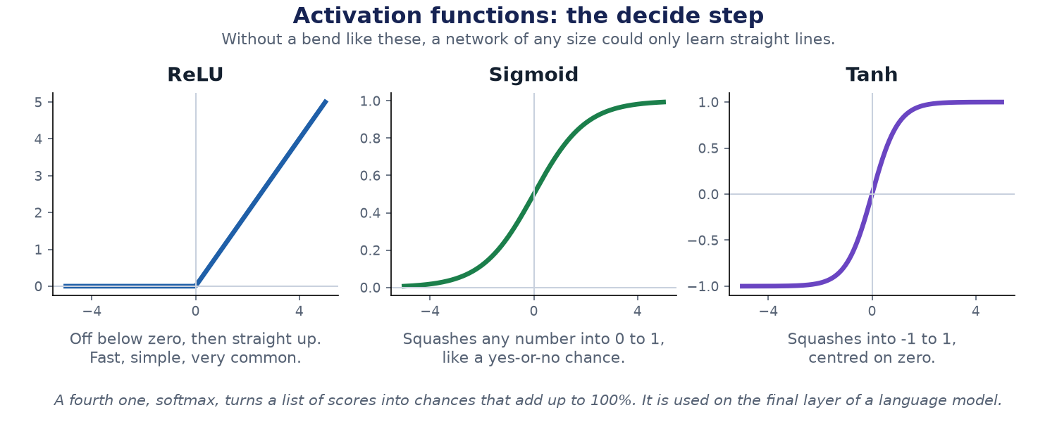
• ReLU is simple and fast, and the most common inside networks.
• Sigmoid squashes any number into 0 to 1, handy for "how likely is it?"
• Tanh squashes into −1 to 1.
• Softmax turns a list of scores into shares that add up to 100%. It is used at the end of a language model to choose between thousands of possible next words.

What can go wrong

• Vanishing gradients. In a very deep network, the blame can shrink to almost nothing as it is passed back through many layers, so the first layers barely learn. Better activations, shortcuts between layers and careful starting numbers fix most of this.
• Exploding gradients. The opposite: the blame grows until numbers overflow. A common fix is to cap the size of the gradient.
• Dead circles. A ReLU circle that always gets a negative total outputs zero and passes no blame, so it stops learning.
• Overfitting. The network memorises the study examples (Chapter 3). More data, simpler networks, and stopping early all help.
• A bad learning rate. Too big and the loss bounces. Too small and nothing seems to happen.

Back to Asha

Asha's photo-recogniser for cakes (Chapter 4) is a network like this, only much larger. Each training step shows it a batch of cake photos, measures the loss, passes the blame back and nudges millions of weights by tiny amounts. After thousands of steps, it recognises a strawberry cake it has never seen. It is the same four steps you just did by hand.

Words explained

• Layer, width, depth: a row of circles; how many circles in a row; how many rows.
• Parameter: any number the network can learn, meaning a weight or a nudge (bias).
• Loss: one number for how wrong the network is.
• Gradient: how much the loss changes if one weight is increased a little.
• Backpropagation: working out all the gradients by passing the blame backwards.
• Learning rate: the size of each update step.
• Batch, epoch: a small group of examples; one full pass through all examples.
• Optimiser: the rule for turning gradients into updates, such as Adam.
• Cross-entropy: a loss for choosing between classes that punishes confident mistakes.

The limits of this chapter

• The network here is tiny and uses the simplest loss and the simplest activation, so you can follow every step. Real networks have many more kinds of layers.
• The numbers were chosen to be easy. Real training starts from random numbers and takes many steps.
• Knowing the steps does not mean we understand why a trained network gives a particular answer. That is still a hard, open problem.

For engineers

• Layer computation: a = activation(W x + b). For a layer with n inputs and m outputs, W is an m × n matrix, so the parameter count is m × n + m. Frameworks compute this in batches as matrix multiplications.
• Backpropagation applies the chain rule. For the loss L, the gradient with respect to a layer's input is Wᵀ times the gradient arriving from above (multiplied by the activation's derivative), and the gradient with respect to W is that arriving gradient times the layer's input. Frameworks do this automatically (automatic differentiation).
• Common losses: mean squared error for regression, cross-entropy on softmax outputs for classification. Common optimisers: SGD with momentum, Adam and AdamW. Learning-rate schedules (warm-up, decay) are widely used.
• Remedies for unstable training: initialisation schemes matched to the activation, normalisation layers, residual connections, gradient clipping, and mixed-precision arithmetic with loss scaling.
• You can reproduce the worked example with a few lines of plain Python. It prints "output 0.8 loss 0.04" and then "after one step: output 1.0225 loss 0.000505".

x1, x2 = 1.0, 2.0
w11, w21, b1 = 0.5, 0.25, 0.0     # into hidden 1
w12, w22, b2 = -1.0, 0.5, 0.5     # into hidden 2
v1, v2, c = 0.6, 0.4, 0.0         # into the output
target, lr = 1.0, 0.1

def forward():
    z1 = x1 * w11 + x2 * w21 + b1
    z2 = x1 * w12 + x2 * w22 + b2
    h1, h2 = max(0, z1), max(0, z2)          # ReLU
    return z1, z2, h1, h2, v1 * h1 + v2 * h2 + c

z1, z2, h1, h2, out = forward()
print("output", round(out, 4), "loss", round((out - target) ** 2, 4))

d_out = 2 * (out - target)                    # slope of the loss
g_v1, g_v2, g_c = d_out * h1, d_out * h2, d_out
d_z1 = d_out * v1 * (1 if z1 > 0 else 0)      # blame passed back, through ReLU
d_z2 = d_out * v2 * (1 if z2 > 0 else 0)
g_w11, g_w21, g_b1 = d_z1 * x1, d_z1 * x2, d_z1
g_w12, g_w22, g_b2 = d_z2 * x1, d_z2 * x2, d_z2

v1, v2, c = v1 - lr * g_v1, v2 - lr * g_v2, c - lr * g_c
w11, w21, b1 = w11 - lr * g_w11, w21 - lr * g_w21, b1 - lr * g_b1
w12, w22, b2 = w12 - lr * g_w12, w22 - lr * g_w22, b2 - lr * g_b2
out = forward()[-1]
print("after one step: output", round(out, 4), "loss", round((out - target) ** 2, 6))

Check yourself

• What does the gradient of a weight tell you? Answer: How much the loss would change if that weight were made a little bigger. A negative gradient means increasing the weight would lower the loss.
• Why is backpropagation called "back"? Answer: It starts at the error at the output and passes the blame backwards, layer by layer, to work out every gradient without trying each weight separately.
• In the example, why did the loss fall so much in one step? Answer: Every one of the nine numbers was nudged in the direction that lowers the loss, and together those small nudges moved the output from 0.8 to about 1.02.